Shock Wave Theory – Rifle Internal Ballistics, Longitudinal Shock Waves, and Shot Dispersion

Introduction

I started looking at the causes of shot to shot dispersion after getting serious for the first time with loading for accuracy. I ran across Dan’s site (green788) and the concept of OCW. I was intrigued by the undeniable fact that a single load recipe can work so well across many different rifles, with different barrel lengths, diameters, and bedding methods. I started reading everything I could get my hands on regarding barrel vibration and the internal ballistics of a rifle during the firing event. The singular thing that I could not get past was that a simple harmonic vibration pattern could not explain the fact that a single load could work with so many different rifles.

I am a radio communications electronics engineer by profession, and deal with resonance and vibration all the time with antennas and other circuits. It is physically impossible for all the different rifles to have exactly the same harmonic pattern with relation to the bullet exit time. Even a simple change in a barrel contour for a given length will change the resonance, much less a change from a 24” tactical barrel to a 27” target barrel. I am compulsive in the fact that I HAVE to have a clear model and theory of why something works before being comfortable with it. I do bow to expediency often, and just use a process or a machine without questioning how it works, but for anything that I am trying to understand and improve on, I have to have a good model.

Observations and the Resultant Questions

So, I started thinking about other possible reasons for the dispersion of shots within a string. During literally thousands of very careful load charge and seating depth experiments, some notable things were observed:

 

1. The point of impact (POI) moved slowly around as the load was increased, the basic premise of Dan’s OCW method.
2. The size of the group or the dispersion around that POI varied VERY quickly as the seating depth was changed.
3. The velocity deviation of a load would varied VERY quickly as the seating depth was changed.
4. Optimum loads work across multiple rifles, with different length barrels.

 

Even 0.3 grains difference in a 25 grain .223 AI load was enough to take it from a 0.5 MOA group to a 1.2 MOA group. Keep in mind these were not single three shot groups, but typically 2 or more groups of 5 shots each at each load condition to validate the measurement. When I looked a keeping the load constant and changing the seating depth, I saw the same very quick changes in dispersion. As little as 0.010” sometimes affected the groups by the same amount as previously described. The velocity deviation changed rapidly as well. I often observed a reverse correlation between velocity deviation and groups size during these experiments, where loads producing good groups had a high standard deviation of velocity, and vice versa. This was not always the case, in fact, once a truly OCW load was achieved, it became quite tolerant to these changes with respect to dispersion and velocity deviation, again validating Dan’s premise.

Here is what drove me nuts for weeks:  A charge change of 0.3 grains or a seating depth change of 0.010” changes the velocity very, very little, usually less than 50 FPS at a mean velocity of around 2900 FPS. The change to the groups, on the other hand, was dramatic.

Why? ? ?

Harmonic Resonance Theory – Does it Fit ?

The first theory is the possibility that the bending modes of the barrel are getting excited differently each shot. Upon further thought, I concluded that this is not possible, based on the following reasoning. The basic resonant (beam bending or “ruler on the edge of the desk”) mode of a cantilevered barrel (beam) made of steel at our typical lengths and diameters is on the order of 500 to 1000 Hz, give or take. Even if you look at higher order modes, such as the 5^th harmonic mode, you are still between 2500 to 5000 Hz. Keep in mind these modes are in reality definitely NOT simple beam bending modes, but have a lot of twisting and elongation going on at the same time as well, a very complex situation. At 5000 Hz, the muzzle (assuming it was at a point of maximum movement) would make one cycle every 1/5000 or 0.2 mS. If the dispersion was due to these beam bending modes, then it should be fairly insensitive to small changes in charge and seating depth. Also, changing the barrel mass distribution even a little will completely change the node position, and therefore make it impossible for a universal OCW load to exist. Therefore, I concluded that the sensitivity to small changes was not from changes in the bending modes.

A Theory to Fit #1

Having said this, I do agree that the POI changes are primarily due to the bending modes, but because they are so low in frequency, they are “smooth” and do not change rapidly over load variations. I can explain this better using an RF engineering analogue. The barrel is akin to a low pass filter, taking the mechanical input from the chamber pressure profile, and “filtering” it through a complex resonant structure to arrive at a muzzle position and bore exit angle time variation. The pressure pulse is quite fast, reaching max pressure in around 0.4 mS typically, with lots of little “bangs and clangs” going on as the firing pin strikes the primer, the primer explodes, the pressure starts to rise and move the bullet, the bolt slams back, and the bullet engages the rifling. All of this happens in well under 0.1 mS (100 microseconds). The mass of the barrel precludes this very fast excitation from getting to the muzzle in any significant amount. It will start to “ring” but won’t get really shaking until the bullet has left. This filtering makes the muzzle position very insensitive to the charge and seating depth.

This model of a bending and vibrating barrel explains the first observation above, and why an OCW load works, as it means that the charge/bullet combination has a very consistent pressure profile, and tends to excite the bending modes in a very regular way, keeping the POI fairly constant.

However, since it ruled out the bending modes out as an explanation for the variation in dispersion and velocity deviation, I was still left with no model for these observations.

Epiphany

Two things came together for me at about the same time, making a unified model possible. First, I read on one of the shooting forums a post from a benchrest fellow about a barrel that he had that was his best ever shooter. He had slugged the barrel, and found that the muzzle was just ever so slightly smaller than the rest of the bore, on the order of one or two ten-thousandths as I recall. His theory was that this was the best possible case for a clean exit, as the bore constriction ensured no gas blow by. Secondly, I remembered one visit to a very tall TV tower in central Maine many years ago. I was killing time waiting for some event to happen (I don’t remember what) and was playing with some truly immense guy wires keeping the 1400-foot tower up in the clouds. These wires were about 3 inches in diameter, and were at least 1000 feet long, and under tremendous tension. I remember grabbing the wire near the dead man anchor, and giving it a shake as hard as possible. I watched the s-shaped wave disappear into the overcast, only to appear a few seconds later, hit the anchor point, can go back into the clouds, and so on until it died out. I played with this like a 2 year old for quite a few minutes. Later on, as an RF engineer, I built many circuits that used sections of transmission line to delay and shape pulses, just like the pulse on the guy wire. Now, guy wires, RF transmission lines, and rifle barrels are very different things, but physics is physics, regardless of the field of use.

Traveling Wave Theory

Here is the second and crucial part of the model:

The pressure pulse from the gasses in the chamber cause a traveling wave of stress that bounces back and forth along the barrel between receiver and muzzle, slightly changing the bore diameter in the process. Minimum dispersion of the shots will result when the rate of change of the bore diameter is at a minimum, and this dispersion will present the least sensitivity to load variations (charge, seating depth).

It is the position of this wave and its effect on the muzzle at the point of bullet exit that is the cause of the majority of the dispersion around the mean POI.

Stress Waves

Treat the barrel as a “conductor” of sound or applied stress, and imagine for a moment that it is infinitely long. If you bang on your section of the barrel with a hammer, it will generate an acoustic or stress wave in the steel, which will travel in both directions away from the hammer impact point at the speed of sound in the barrel. The stress wave is a wave of force on the steel, some of which is in the radial (in and out from the bore across the direction of travel) direction, called a transverse stress component, and some of which is in the direction of travel, called a longitudinal stress component. An acoustic wave in air is primarily longitudinal, where the air compresses and expands along the direction of travel. In a solid, such as steel, both components can exist at the same time. In our infinite barrel, the wave travels on and on until the mechanical losses in the steel dissipate the stress energy as heat.

Reflections

However, we do not shoot infinitely long barrels, so what happens to the stress wave in a real rifle barrel? Just like in the TV tower guy wire, if a stress wave reaches a mechanical discontinuity in the object it is traveling in, such as the muzzle end of the barrel, or the solidly bedded receiver end of the barrel, it will reflect back in the opposite direction. In steel, the speed of sound is very close to 0.227 inches per microsecond, or about 18916 FPS. A wave will travel from the receiver to the muzzle in the barrel in about 0.12 mS. It can make around 4 or 5 round trips before the bullet leaves. Note that it does not matter how heavy the barrel is, or the profile, as the wave travels at almost exactly the same speed in all cases.

Stress Causes Strain or Distortion of the Muzzle – Explaining Observation #2

What does this stress wave do? Remember that stress is the amount of force or pressure applied to a material, which usually results in the material moving, bending, or displacing. This is called strain. So, the pressure stress from the gasses in the chamber causes a resulting strain in the barrel. Because the stress is applied very rapidly, the some of the stress launches down the barrel as a wave, causing a proportional strain to the barrel as it passes. This strain is initially a slight enlargement of the bore, followed by a slight constriction, eventually dropping off to no change in the bore diameter at all.

As this pulse travels to and fro, it passes by itself, and in the process constructively and destructively adds to itself, all in some predictable way. The shape of the pulse is driven by the pressure/time profile from the propellant burn, and the mechanical properties of the barrel. The theory nicely provides an explanation why very small changes in load parameters could result in large changes in dispersion. If the muzzle diameter is changing very rapidly at a particular time after shot initiation, and if the bullet exits at this time, then very small changes in the load will result in small changes in the exit time, but large changes in the exit direction since the muzzle diameter is always different. Think of this as a dynamic variation of the muzzle crown shape. It is well known that the crown is perhaps the most critical part of the barrel as regards accuracy. So, this theory or model can explain the sensitivity to the load, and explain observation #2 above.

Model and Simulation

Nice theory, but where is the proof? To prove a theory, you have to first make a model that can (hopefully) predict the behavior of the real system, and then use that model to predict the outcome of some controlled experiments. If the experimental data fits the model data, then you can at least say that the test did not disprove the theory.

To test this theory, I constructed a model of a rifle barrel using Matlab. Matlab is a very powerful engineering programming and analysis tool, and is perfectly suited to this sort of analysis. I used a simple filter model of the barrel to predict how the stress wave would look when excited from a perfectly sharp hammer blow, or unit impulse. This is shown in Figure 1 below.

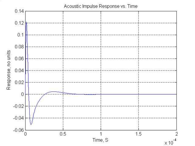
Figure 1 - Acoustic Impulse Response

The pressure versus time curve was taken directly from a Quickload analysis of my accuracy load for my .223 Remington Ackley Improved with a 27” barrel. This is 75 grain Hornady AMax over 25.5 grains VVN140, at about 2950 FPS. The pressure curve is shown in Figure 2.

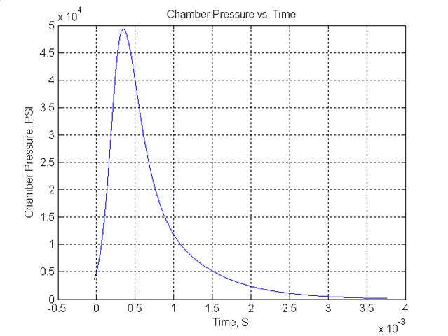
Figure 2 – Chamber Pressure versus Time

Now here the model gets a bit complicated. In reality, the pressure does not stay in the chamber, but actually follows the bullet as it travels down the bore. To make this first simulation computationally tractable, I made the assumption that the pressure pulse was always concentrated at the chamber end, and did not take into account the bullet movement. Future versions of this simulation will include this effect. However, this is more than good enough to get a first order look at the system. So, if you take the pressure pulse and pass it through the filter (barrel) that has the impulse response shown in Figure 1, the resulting traveling stress wave looks like Figure 3.

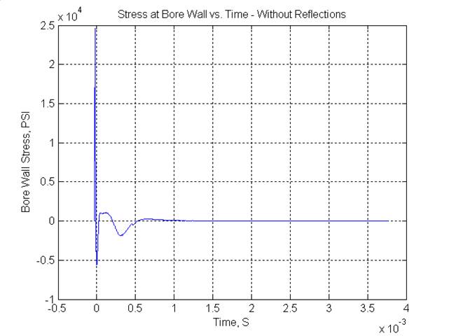
Figure 3 - Bore Stress  versus Time

Figure 3 shows the stress wave as if the barrel were infinitely long. Of course, this is not the case, so we have to make the model simulate the effect of this wave reflecting back and forth. Notice that the pulse has some interesting “tail” responses about 0.5 mS after the main disturbance. These are due to the differentiation of the main pressure peak by the barrel response, and turn out to be the most significant feature of the whole system.

The simulation computes the addition of this pulse at every point in the barrel, at every time point in the simulation. Matlab can even animate the pulse as it travels to and fro. The barrel length, while 27” from bolt face to muzzle, is actually only as long as about the middle of the chamber to the muzzle, from this pulse point of view. Until I get a chance to electronically instrument a barrel, I will continue to use this as my effective barrel length. This is just a guess and a convention, but is subject to change until more data is accumulated. So far, this assumption is holding up.

However, we are most interested in the stress at the muzzle as time progresses. A plot of the muzzle strain (diameter change) as a result of this stress is shown in Figure 4. Again, please remember that this is a simple simulation of the muzzle strain, and does not include the harmonic vibrations, recoil, or other disturbances that occur in the real world.

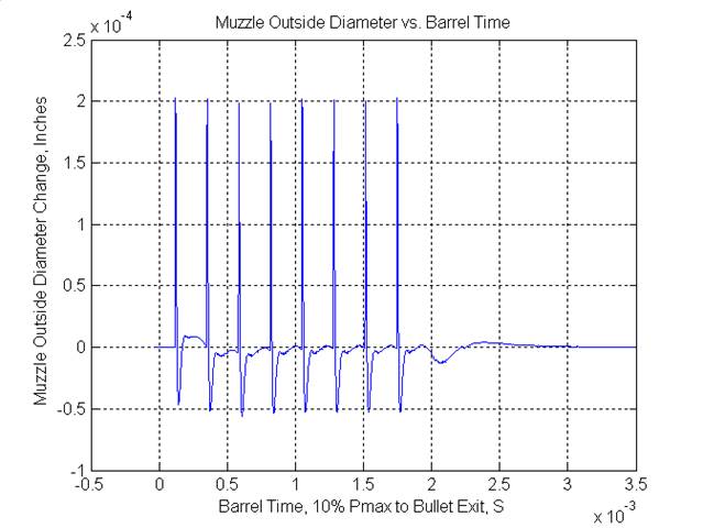
Figure 4 - Muzzle Bore Diameter Change versus Time

Notice that the simulation carries on even after we know the bullet has exited, in case at about 1.24 mS according to Quickload

Zooming in around our exit time, we can see that the muzzle has some interesting behavior in this area of time, Figure 5.

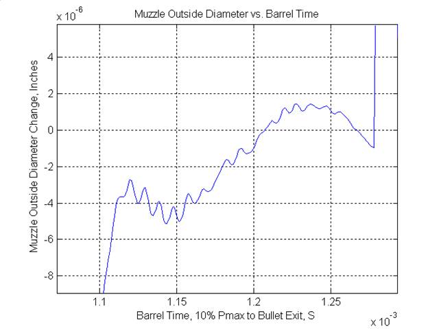
Figure 5 - Muzzle Disturbance at Bullet Exit Time

A Theory to Fit #2 and #4

The theory states that if the bullet leaves at the time when the rate of change of the muzzle diameter is minimum, the dispersion will be at a minimum, and any small variations in exit time caused by load variations will have a minimum effect on the dispersion. Notice that the bullet exits (1.24 mS) right when the rate of change in muzzle diameter is at a minimum. Also notice that at around 1.05 and 1.28 mS, the pulse is right at the muzzle, and the diameter is all over the map. In fact, the best spot is (for this particular round trip cycle) at 1.24 mS, or just before the pulse comes back again. There is another, not as wide in time, sweet spot at about 1.15 mS.

Therefore, this theory and model seems to predict the optimum exit times based on barrel length alone, where the group dispersion is at a minimum. This supports observation #4 above.

Optimum Barrel Times

The simulation was used to predict the optimum bullet barrel dwell times (10% Pmax to exit) as a function of barrel length, as shown in Table 1:

Optimum Barrel times vs. Barrel Length - Node Number as Parameter
Barrel Length, Inches
node #	16	17	18	19	20	21	22	23	24	25	26	27	28	29	30
1	0.550	0.580	0.610	0.645	0.670	0.700	0.790	0.810	0.825	0.855	0.883	0.915	0.940	0.970	1.000
2	0.590	0.640	0.680	0.720	0.760	0.775	0.840	0.870	0.900	0.945	0.978	1.005	1.035	1.060	1.090
3	0.685	0.725	0.765	0.805	0.840	0.880	0.980	1.005	1.030	1.070	1.110	1.150	1.185	1.220	1.260
4	0.725	0.785	0.835	0.880	0.930	0.955	1.030	1.065	1.120	1.160	1.200	1.240	1.275	1.310	1.345
5											1.330		1.425	1.470	1.520
6														1.560	1.605

These times were obtained by running the simulation at each barrel length, the visually determining the time of least muzzle diameter change for each round trip.

One of the major observations was that OCW loads tend to work well in almost any rifle, regardless of barrel length. This observation forced us to abandon the concept of a simple harmonic vibration as being the cause of dispersion. So, how does a given load (bullet, case, powder, and specific charge weight) work if we use that same load in rifles with different barrel lengths?

The accuracy load developed for the .223 AI 27” rifle was used as the constant in Quickload, and the barrel time was computed in Quickload after changing only the barrel length. This was plotted against the model simulation of the muzzle disturbance over the same length of barrels, with the best exit time chosen for each length, for the same round trip number. Figure 6 shows this data. The blue line with diamond markers shows the relationship, with each marker corresponding to a particular barrel length. The 16” length point is the marker to the far left, and the 27” length point is at the far right. It is nearly a straight line, as expected. However, it does not track exactly one for one with barrel length, and shows some divergence as the length is shortened. The purple line is what an exact one for one relationship would be. It is interesting to note that the relationship is very close to one to one from about 24” to 27”, the length range that in which the vast majority of bolt action rifles are produced. This shows that the ability of an OCW load to work well across many rifles is supported by this theory and model.

Figure 6 – Quickload Predicted Barrel Time for Given Load as Compared to Predicted Optimum Barrel Time

A Theory to Fit #3

So, we now have a model that supports observations #1, #2, and #4. What about observation #3? Can it explain the extreme sensitivity to seating depth of the group size and the rapid changes in velocity deviation?

Bullet Modulation

I believe the theory does explain this sensitivity, for the following reason. Since the pulse is changing the bore diameter as it passes back and forth, it seems reasonable that the bullet frictional load is also changing as the bore diameter changes. During the first two or three trips back to the chamber end, the bullet has moved by less than two inches, and the pressure is at or near maximum, Figure 7. If the bore constricts, it will cause the bullet to be retarded some, and thereby increase the pressure rate of increase. Conversely, as the bore expands after the first part of the pulse passes, the bullet will be looser, and the pressure increase rate will drop. In other words, the pulse, by interacting with the bullet during the critical first few inches, can dramatically change the burn characteristics by modulating the bullet retardation forces.

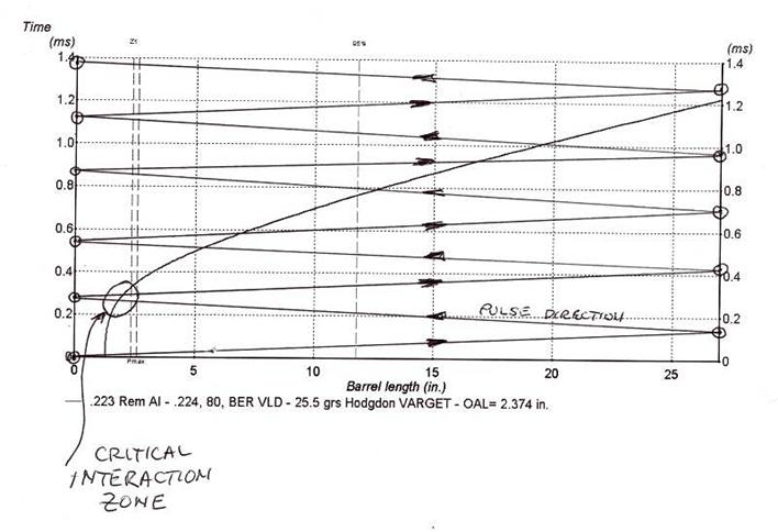
Figure 7 - Pulse Reflection Superimposed over Bullet Position versus Time

To understand this, we need to look at how propellants burn in a cartridge. Propellant burn rates are controlled by many factors, but in general they burn faster at higher pressures and slower at lower pressures, especially in the initial stages of combustion. During the initial stage, the powder is not all lit, and the flame front is moving out to all the grains. In the intermediate stages, all the grains are lit, and gas is being produced at a rate that is a function of the pressure and temperature and the powder characteristics. In the final stages, the gas production rate is dropping off as the grains become consumed.

Any systematic effect that varies the chamber pressure or volume during the initial stages can dramatically change the pressure peak time. If a load is not very heavy and the case is not very full, the initial stages last longer than in a load that is near max. All the OCW loads developed with this theory have been found to work best when the powder charge is near max volume for the case and bullet combination. This also explains why variations in neck tension and seating depth can have an (sometimes) adverse affect on accuracy and velocity variations. Granted, this is not at all new, but now there is a consistent explanation for why this is so.

The modulation in pressure by the interaction of the reflected pulses and the bullet will slightly change the position of the bullet on the next pulse pass, further changing the burn. The nest result is that the overall burn becomes chaotic, which by definition is any process that exhibits extreme sensitivity to initial conditions. On the other hand, if the timing of the pulse over the bullet is after the powder reaches the intermediate point, then the modulation effects become less significant.

So, the reason why we see very significant group size changes by changing the seating depth (question #2 above) can now be explained by the interaction of the pulse with the bullet during the initial stages of propellant combustion. The rate of burn, and hence the actual barrel time will be varied a lot by small changes in the amount of time it takes for the pulse to comeback over the bullet. Question #3 is also explained simultaneously as #2, since they are really one in the same, as changes in barrel time result in changes in muzzle velocity. We need only to be sure that we choose a powder and charge volume that insures that the powder is out of the initial stages before the first return trip of the pulse.

Comparing Model Predictions and Real World Range Results

So, how does this model hold up to the real world? In a word (well, two words), almost perfectly. I say almost, since there is enough error in Quickload and in the ability to estimate the precise effective barrel length that the actual power charge needed for optimum groups was usually about 1 to 2 percent less than Quickload predictions. Note that Quickload uses the time from 10% of maximum pressure the bullet exit as the definition of barrel time. I have adopted this as my definition in order to keep my use of Quickload as simple as possible.

Even given these potential sources for modeling error, I was able to validate that the optimum barrel time for this 223AI rifle with its 27” barrel is right at 1.24 mS, for multiple powders. Since I could not get the 75 grain bullets to exit in 1.15 mS without greatly exceeding the maximum pressure, I tried using 55 grain Vmax bullets, and again had minimum groups sizes at exactly the expected barrel time of 1.15 and 1.05 mS. I noticed that the load sensitivity here was higher than at the slower load, which is predicted by the narrower stable time period at 1.15 mS. See Table 2 and Table 3. These tables document the loads used to validate the model with 75 and 80 grain bullets, my primary desired projectiles for this project rifle. They show the measured group sizes, velocity performance, and the predicted data from Quickload. All loads were shown to provide the best groups and minimum POI shift, over the widest variation in charge weight and seating depth. They are true OCW loads.

Table 2 - .223 Remington Ackley Improved Optimum Load Data - Original Throat