Group Size Statistical Analysis

 A PDF version is here

The relationship between a rifles inherent accuracy and the size of a group it can shoot at a specific range is very interesting. This article shows this relationship in a way that clearly connects the accuracy of the firearm to the size of the groups it will produce. A table is presented to allow a shooter to estimate the actual Minute Of Angle (MOA) accuracy of the firearm from one or more groups. The overriding assumption of the following discussion is that we are dealing with a very simple statistical model, one that does not take into account all the common factors that cause a variable shot to shot dispersion, such as the shooter, ammo, wind, unbalanced bullets, etc.

Most Common Method Used to Determine Group Size

By far the most common method for measuring the accuracy of a given rifle is to shoot a few groups of some number of shots each, and measure the average of the distance of the two shots in each group that are the farthest apart. The assumption we will follow here is that this is done at a standard range of 100 yards. Then the shooter will convert this distance to MOA using the approximation of 1 MOA = 1 inch @ 100 yards.

For example, given the target shown below in Figure 1, for 3 shots @ 100 yards:

Figure 1 - Typical group measurement method

Here this three shot group would be said to have a group size of d inches, as measured from the center-to-center distance between the two farthest spaced shots. If, for example, this measured to be 0.75 inches, it would normally be said that this is a 0.75 MOA group. Note that the US Military uses the measurement of the mean radius of all the shots in each group as the definition of the angular accuracy of a given firearm, not this “extreme shot distance” measurement.

There are a number of assumptions that should be noted when using this convention; these are detailed as follows.

Inches, MOA, and MILs – Measurement of the Angle of Shot Dispersion

For a target at 100 yards, an angular spacing of 1 MOA, or 1/60 degree is very close to, but not exactly one inch:

Another measurement that is commonly used is the Mil, short for milliradian, or one thousandth of a radian. There are 2*PI radians in 360 degrees, so a milliradian is equal to:

Therefore, it is a valid approximation to equate a one inch distance at 100 yards to 1 MOA. We will use this approximation for the remainder of this article. If the reader desires to measure in MILs, we will leave it up to the reader to perform the appropriate conversions.

Accuracy and Repeatability

Most shooters will refer to the group size as an indicator of the accuracy of the rifle, while in fact it is really an indicator of the repeatability of the rifle.

A shooter will fire a group at a particular Point Of Aim (POA), and the resulting group center or mean Point Of Impact (POI) will usually be offset somewhat from the intended POI or the POA. This offset is an indicator of the accuracy of the rifle, since it is this bias that must either be removed using the scope adjustments, or by applying an offset “hold” when firing a shot. Assuming that the scope can be adjusted appropriately, or the shooter can consistently hold off the POA by the necessary amount, then this will be the most probable POI for any given shot. This accuracy can be affected by many variables, such as variations in the charge weight, ignition and burning rate, bullet consistency, barrel and action heating, and wind. We will ignore these effects for the remainder of this article.

Once a given POI is established, a group of shots will be distributed around the mean POI in a (usually) random fashion. The size of this distribution is the repeatability of the rifle. This is what has been described above as the group size. An important assumption here is that we are ignoring many real-world effects such as shot-to-shot velocity variations (causing a vertical dispersion which is added to the random distribution), and that of wind (causing a horizontal dispersion which is added to the random distribution), as well as many others.

A truly accurate rifle will have a precise and repeatable POI and a small distribution of shot impacts around that point.

Gaussian Distribution – A Simple Model of How Shots are Dispersed

Another major assumption we will make in this article is that the above mentioned dispersion of shots around the POI is distributed in some known fashion.  We choose to use the normal or Gaussian distribution model. This is the famous “bell curve”. Obviously, it is impossible to determine if any given rifle or load for that rifle will have a true normal distribution of shots around the POI. However, through a lot of observations and lead thrown downrange the author has found this model to fairly accurately describe group distributions for most rifles and loads.

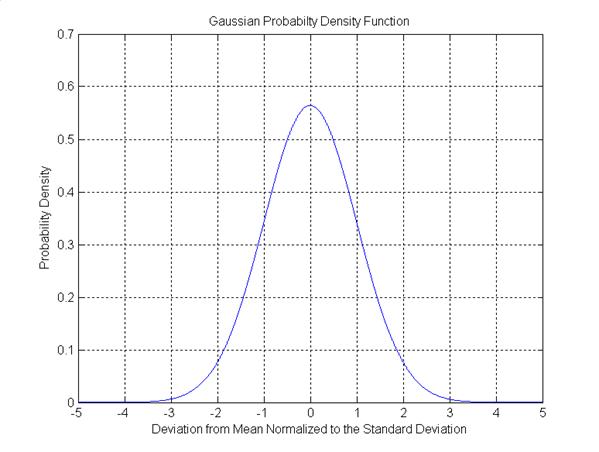
Figure 2 - Gaussian (Normal) Probability Distribution

Figure 2 shows the double-sided Gaussian distribution as a probability density. The X axis is the offset from the mean in units of standard deviations. The area under this curve is identically equal to one. A standard deviation defines a specific deviation from the mean (a mean of zero in this case) that can be expected a certain percentage of the time. This means that if a process has this distribution, 68.2% of the time the value will fall between -1 and +1, 95.5% of the time between –2 and +2, and 99.7% of the time between –3 and +3.

We can apply this to our shooting model by defining the accuracy of our model as the angle in MOA of the standard deviation for the projectile from the true flight path.

Figure 3 - Shot Deviation Angle

Figure 3 shows the deviation angle as the deviation away from the perfect (straight) path. We wish to define our model such that this deviation angle (cone angle) has the distribution shown in Figure 2, and that each shot will exit at a random angle with equal probability around the perfect path (clock angle). Figure 4 illustrates this definition.

Figure 4 - Definition of Cone and Clock Angles

Since most shooters use the distance between the two farthest shots in a given group, we need to define the angular (cone angle) standard deviation of our model as the double-sided standard deviation. This means that the standard deviation of the cone angle shown in Figure 4 will be one half of the desired angular deviation. As an example, if our imaginary rifle had a double sided standard deviation of one MOA, then 68.2% of the time a shot will fall within a one inch diameter circle at 100 yards, centered at the actual mean POI.

The Simulation and Some Results

A Matlab program was written that simulated 100000 shots from a rifle, with a one MOA double sided standard deviation of cone angle, at a target 100 yards away. The simulation then formed as many groups of N shots as it could from the total of 100000, and calculated and recorded the largest center-to-center distance of each group of N. N ranged from 2 to 20 shots. It then averaged all the group sizes recorded for each N, resulting in the average group size for a N shot group. For example, given 100000 shots, there were 5000 groups of 20 shots. This resulted in 5000 group size measurements, and one average group size value for a 20 shot group.

Figure 5 shows a simulated target after 250 shots. The rings are spaced 0.5 inches apart. Notice that most of the shots fall within a one inch circle, but there are only a few that are more than one inch away from the mean POI. In fact, the center regions of the target are hit most frequently, and with far fewer hits at the edges of the target.

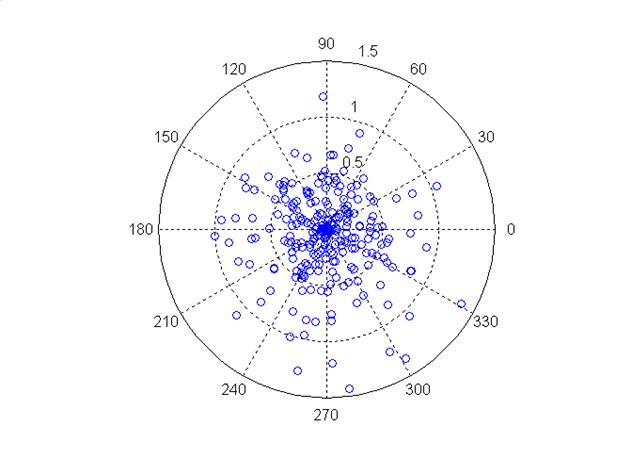
Figure 5 - Simulated Target After 250 Shots

A histogram showing the distribution of the shot impact locations for the above conditions is very interesting and is shown in Figure 6. The spike shows clearly that a shot is most likely to land in the center, with shots far away from the center occurring much less frequently. This result shows clearly that one could shoot two or more three shot groups with a small (say 0.5”) group size, then have another 3 shot group exhibit two shots very close to each other with a third shot landing an inch or more away. The distribution shows only the probability of a single shot falling at a point away from center, not the probability of a group of shots falling at a particular distance. This explains why one may see unexplained “flyers” out of a good shooting rifle. These are not true “flyers” in the sense that some process other than the normally distributed angle deviation caused them to diverge significantly, such as a damaged crown or an unbalanced bullet, but are the result of the characteristics of the shot angular distribution itself.

By intuition, it is obvious that a total aggregate of three shots is clearly not a large enough sample size to accurately determine the true distribution of a rifle and load. The lesson here is to shoot many shots, usually in multiple groups of five, and average these to get the aggregate. Just how many shots are needed to form an accurate estimate requires a deeper mathematical analysis of the underlying statistical model, and will be the subject of a future paper.

Based on these conclusions, the author uses 4 groups of five shots for the final proofing of a load.

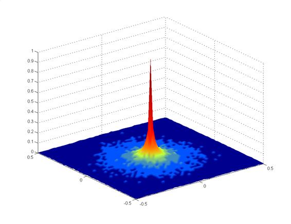
Figure 6 - Target POI distribution for 100000 Shots

Now that we have simulated the perfect one MOA rifle, how does the group size measured for a particular number of shots per group actually correspond to the one MOA accuracy? The average group size measured for shot groups of 2 to 20 each is shown in Figure 7.

Figure 7 - Average Group Size as a Function of the Number of Shots Per Group, 1 MOA standard Rifle at 100 Yards

Notice that if you use three shot groups to determine the actual accuracy, you will observe a 0.863” average group size for a one MOA rifle. In other words, you must measure the average group size in inches, and multiply by the correction factors in Table 1 to get the actual MOA accuracy for the rifle. Remember that this example assumes a 100 yard target range. For ranges other than 100 yards, one can scale the value obtained from the group size measurements after correction by the factors in Table 1 by the ratio of the actual range to a standard 100 yard range. A fairly accurate way to do this measurement without calculation is to use 4 shot groups, as the correction factor is closest to one (0.979).

Table 1 – Group Measurement Correction Factor

The equation below summarizes the measurement and correction process:

For example, your rifle averaged 0.75 inch 5 shot groups at 200 yards. The correction factor from Table 1 for 5 shot groups is 0.876. Therefore, your rifle is shooting at 0.75 X 0.876 X 100/200 = 0.329 MOA.